Cosinor Calculation:
The formula for Cosinor is:
Y(t) = M + Acos(2πt/τ + φ) + e(t)
Y(t) or Yi -- data collected at times ti (i=1, ... , N)
M -- MESOR (midline estimating statistic of rhythm)
2A -- double amplitude (a measure of the extent of predictable change above and below the midline within a cycle)
φ -- acrophase (a measure of the timing of overall high values)
τ -- period (duration of one cycle)
e(t) or ei -- the error term at each time. Assumed to be independent, normally distributed, with mean zero and unknown constant variance sigma squared.
When the period is known, the model can be rewritten as
Y(t) = M + βX + γZ + e(t)
where β = Acosφ ; γ = -Asinφ ; X = cos(2πt/τ) ; Z = sin(2πt/τ)
The model is linear in its parameters M, β and γ.
The regression analysis method of the least squares can be used to find values M, β and γ such that the residual sum of squares Σi e2 is minimal, or equivalently its first-order derivative is equal to zero. To obtain the system of equations for use in this regression, differentiate Σi e2 with respect to each parameter , equating each derivative formula to zero. The resulting system of equations is shown below.
Solving the system of equations thus obtained for the parameters M, β and γ can be done with matrix algebra, or using a linear model function. The following demonstrates the method for solving by matrix.
System of equations:
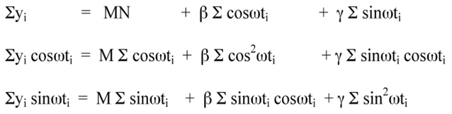
System of equations, where ω=2π/τ
Matrix form:
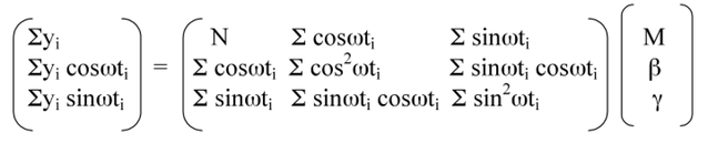
Matrix form: b = S x
Solving for M, β, γ
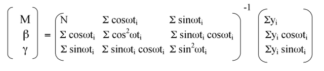
Estimates of M, β and γ are obtained by inverting the S matrix: x = S(-1) * b
To calculate the estimate for Amplitude and Acrophase:
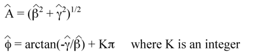
The proper calculation of Acrophase (φ) must take the sign of β and γ into account.
For multiple frequencies:

The model extends to include more than a single period length (frequency). Each frequency adds a term to the equation.
A system of 2k+1 normal equations is needed to solve for 2k+1 variables: M, Ai, φi, with periods τi
Excerpted from a Phoenix Presentation powerpoint, Germaine G Cornelissen-Guillaume, University of Minnesota, 2005
As with any mathematical or experimental endeavor, there are fundamental principles that must be followed. Results obtained without adherence to required assumptions cannot be considered valid. For a review of some of the background assumptions required for rhythm analysis and by the Cosinor, see:
Theoretical Biology and Medical Modelling.2014, 11:16
DOI: 10.1186/1742-4682-11-16
ANALYSIS OF RHYTHMS USING R: CHRONOMICS ANALYSIS TOOLKIT (CAT)
More about Cosinor
The single and population-mean cosinor techniques were first developed and extensively applied to analysis of biological rhythms by Franz Halberg, at the University of Minnesota, to handle short time-series and sparse data when prior information is available (Halberg et al., 1967). Its ability to handle non-equidistant and missing data is a powerful feature. Cosinor is a regression technique that fits one or more cosine curves to the data, separately or concomitantly, minimizing the sum of squares of the differences between the actual measurements and the fitted model (the residuals), for the specified period (Halberg, 1980). From this model, one obtains, for the period considered, an estimate of (i) the rhythm-adjusted mean or midline estimating statistic of rhythm (MESOR), defined as the average value of the curve fitted to the data, (ii) amplitude (A), defined as half the height of oscillation in a cycle approximated by the fitted cosine curve (difference between the maximum and the MESOR), and (iii) acrophase (ϕ, a measure of phase), the lag from a defined reference time point (e.g. local midnight, or other significant point) to the crest time in the fitted curve (see Figure 1). Statistical significance is determined for each of the given metrics by an F-test with respect to the null hypothesis (zero amplitude or no-rhythm). Cosinor also reports an estimate of the percentage rhythm, or proportion of variance accounted for by the model (Cornélissen and Halberg, 2005).
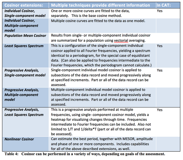
The single cosinor is the core of a set of cosinor-based methods, that calculates the best fit of a cosine model made up of either one, or multiple cosine components, at specified periods. A population-mean cosinor (to be added to CAT) can summarize single cosinor results (either single- or multiple- components models) from a set of individuals at a common time period by vectorial averaging of individual results from the single cosinor, estimating the extent of similarity among individuals (Cornélissen and Halberg, 2005). Additional extensions of the cosinor are listed in Table 4. Those performed by CAT are described further in the coming section.
The single cosinor is the core of a set of cosinor-based methods, that calculates the best fit of a cosine model made up of either one, or multiple cosine components, at specified periods. A population-mean cosinor (to be added to CAT) can summarize single cosinor results (either single- or multiple- components models) from a set of individuals at a common time period by vectorial averaging of individual results from the single cosinor, estimating the extent of similarity among individuals (Cornélissen and Halberg, 2005). Additional extensions of the cosinor are listed in Table 4. Those performed by CAT are described further in the coming section.
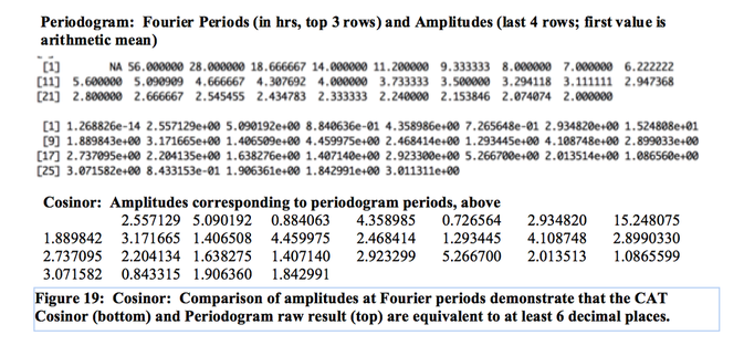
The single cosinor, when used to calculate the Fourier frequencies, yields results identical to a periodogram (Bloomfield, 2000). Figure 18 shows a periodogram calculated with CAT, from equidistant blood pressure readings, with a list of the strongest four periodicities (largest amplitudes). Frequencies corresponding to those on the periodogram are also calculated with cosinor, yielding the same four strongest periodicities, with identical amplitudes, listed below the periodogram. A complete listing of the amplitudes calculated for each period is given in Figure 19. They are identical to 6 decimal places. Bloomfield (2000) proved the equivalence between the discrete Fourier Transform (periodogram) and the regression approach (cosinor).
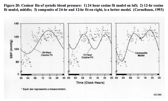
CAT has implemented the single cosinor, with a multiple-components cosinor near completion. The multiple-components model fits a combination of multiple cosine curves of selected period, and can model more complex curves (Figure 20). Cosinor, like all CAT functions, can calculate circadian or other periods, from years to seconds, etc. It can calculate any frequency, not limited to the Fourier frequencies. The single-component cosinor in CAT allows specific frequencies/periods to be selected for any analysis. Any subsection of the time series can be designated for analysis. CAT Cosinor produces both graphical and numeric listings of results.
Reference Time selection: As we have seen, the reference time is important in esimating rhythms. CAT Cosinor allows the user to specify this as a parameter.
Period selection: One or more specific periods can be selected for analysis, or CAT can be instructed to analyze a range of periods. The user can specify a custom range of periods to be calculated, or allow CAT by default to do the calculations for the set of all Fourier periods for the data set, from T/1 (1 cycle per T), to 1/2, ending with the Nyquist. This produces the equivalent of a periodogram, although unlike a periodogram, it can be performed on non-equidistant data. Whenever a range is specified (e.g., 252 - 9.5), an increment can also be considered (e.g., .5), identifying the set of periods to be calculated (e.g., 252/1, 252/1.5, 252/2, 252/2.5… 252/9.5). In this way, the frequencies in a periodogram can be calculated, with the addition of intermediate frequencies!
When the first period estimated is T (record length in time) and the harmonic increment is 1, the periods correspond to Fourier frequencies. Using a fractional harmonic increment allows estimates of rhythm characteristics at intermediate periods. This is advantageous in identifying the period associated with the largest amplitude (or rather percentage rhythm), even if it is not a Fourier period. It should be remembered, however, that this approach may allow a more accurate point estimate of the period, but it does not improve the uncertainty with which the period can be estimated.
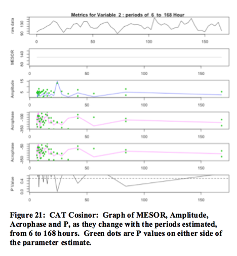
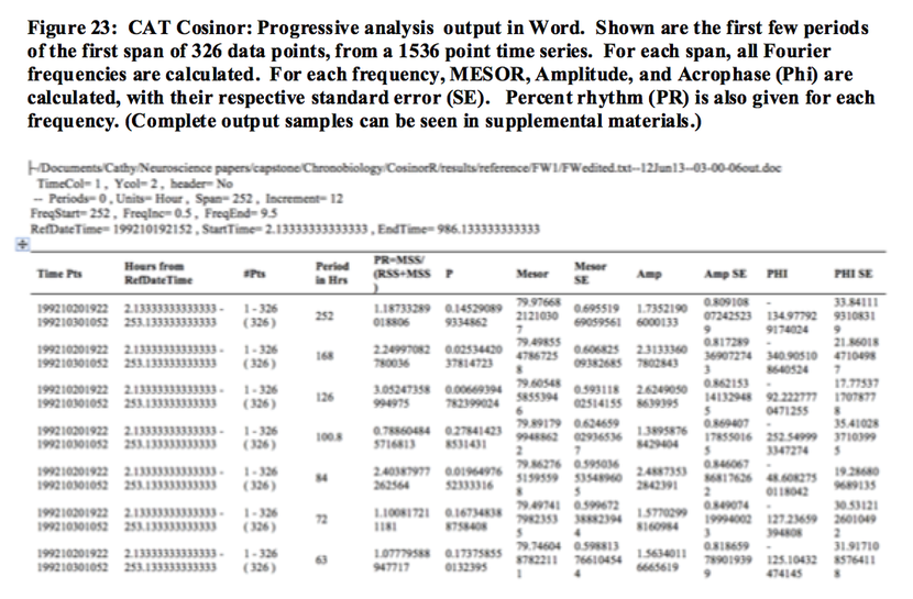
Results: For each period considered, results show the estimates of the MESOR, amplitude, phase, and a standard error for each rhythm parameter. An F-test is used for rhythm detection, yielding the significance level associated with the fitted curve and the corresponding percentage rhythm (R2), for the period assessed. When multiple periods are selected to be analyzed, a graph is produced for MESOR, amplitude, phase and percent rhythm, showing how each varies across the span of investigation (Figure 21).
Time span selection: CAT Cosinor can also be configured to calculate a specified subset of the time series. Any period selection can be combined with any time span selection.
The analysis selected can also be performed on multiple variables in a single run (sequentially) for any range of columns in the input file, where each column is an individual variable, by selecting the columns to be processed. For example, to run an analysis in CAT on systolic blood pressure, diastolic blood pressure and heart rate data columns, where each is a separate data column, select those three input file columns at execution.
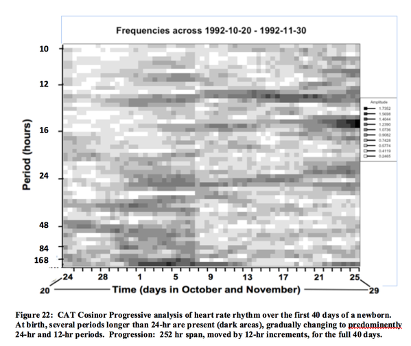
Progressive Analyses: This method, used by other CAT functions as well, allows increased insight into how, or whether, the data series may be varying over time. Progressive analysis breaks a set of data into subsections, or overlapping subsections, and assesses each subsection successively, constructing a heat map of rhythm amplitudes as a function of frequencies over time (Figure 22). Progressive analysis can be performed on single, multiple, or a range of periods. Output, in this case, consists of the table of values as above, in addition to a heatmap, in color or black and white, of the spans plotted over time for each period.
Output formats, and output content can be configured as needed. Options for output formats include: a .txt file, containing a table of rhythm characteristics for each period considered; or a more attractively formatted Word document of the same content (Figure 23). The line graphs (Figure 21) and the heatmap (Figure 22) can be turned on or off as needed. The graphics can be produced in a several formats: PDF, JPG, PNG or postscript (PS). The CAT website details usage.